Computational fluid dynamics
finitevolume-
A small solver. A close look at compressible flow.
Follow a classic shock-tube problem from its initial conditions to a numerical solution. Read the Python code, run the case and contribute to what comes next.
View source code (opens in a new tab)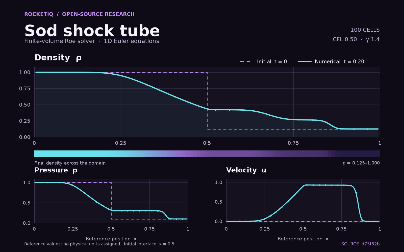
See the physics in the code.
A shock tube starts with two gas states separated by a sudden change in density and pressure. The Sod problem follows the waves that develop from that initial discontinuity, making it a useful case for exploring compressible-flow methods.
This project implements a compact, one-dimensional finite-volume solver in Python. It evolves density, momentum and total energy using Roe’s approximate Riemann solver, then recovers velocity and pressure from that state.
It is a starting point for learning numerical CFD and developing contributions you can reproduce: a readable solver, a configurable reference run and a small set of physical sanity checks.
What is inside the solver?
- Finite-volume formulation
- A uniform, cell-centred grid with first-order updates of the conserved quantities.
- Roe interface flux
- An approximate Riemann solver evaluates the flux between neighbouring cells using a Roe-averaged state.
- CFL-controlled time steps
- The step size follows the largest local wave speed and is shortened to reach the requested final time.
- Fixed end states
- The first and last cells retain their initial states throughout the calculation.
The current implementation is focused on the Sod initial condition and a first-order method. It does not include higher-order reconstruction or an entropy fix. The included tests check this reference case; they do not establish accuracy or robustness for every flow problem.
The reference Sod case
The supplied YAML manifest sets 100 cells, CFL 0.5, a final time of 0.20 and a specific-heat ratio of 1.4. The default domain spans x = 0 to 1, with the initial discontinuity at its midpoint.
| Initial state | Density ρ | Velocity u | Pressure p |
|---|---|---|---|
| Left half | 1.0 | 0 | 1.0 |
| Right half | 0.125 | 0 | 0.1 |
The runner writes a density plot to outputs/density.png and records the command, solver wall time, cell count and final simulated time in outputs/run_log.json. The solver also returns velocity and pressure arrays, which are used in the figure above.
The two included tests check positive final density and pressure, and approximate mass conservation, for this same case. You can inspect both checks in the repository.
Run it on your machine.
You will need Git and Python. The repository’s CI configuration uses Python 3.11. Start by cloning the repository and creating an isolated environment:
git clone https://github.com/RocketiQ/finitevolume-shocktube.git
cd finitevolume-shocktube
python -m venv .venv
Use the commands for your operating system. They call the environment’s Python directly, so activation is not required.
macOS / Linux
.venv/bin/python -m pip install -r env/requirements.txt
.venv/bin/python -m pytest -q
.venv/bin/python -m scripts.run --manifest cases/sod_small.yml
Windows PowerShell
.\.venv\Scripts\python.exe -m pip install -r env/requirements.txt
.\.venv\Scripts\python.exe -m pytest -q
.\.venv\Scripts\python.exe -m scripts.run --manifest cases/sod_small.yml
On systems where Python is available as python3, use python3 -m venv .venv for the environment creation step. Dependencies include NumPy, Matplotlib and PyYAML, with pytest and Ruff for development.
Explore the repository.
Start with the method, follow the implementation and inspect the checks. If you use the project in your research or teaching, refer to its citation metadata.
- Numerical method and assumptions (opens in a new tab)
- Finite-volume solver (opens in a new tab)
- Roe flux implementation (opens in a new tab)
- Reference-case tests (opens in a new tab)
- Sod case configuration (opens in a new tab)
- Citation information (opens in a new tab)
- Apache 2.0 license (opens in a new tab)
Build on what is here
Your next contribution starts on GitHub.
Documentation, tests and numerical improvements all matter. Browse the issues or propose a focused change, then follow the repository’s contribution instructions.
Run the baseline
Fork and clone the repository. Set up your environment, run the tests and reproduce the Sod density plot.
Make a focused change
Clarify a method, strengthen a check or discuss an extension. Rerun the tests and reference case to understand its effect.
Open a pull request
Use the repository’s template. Explain what changed, list the commands you ran and attach the new figure if the results changed.